---
title: "Law of Large Numbers"
---
```{r setup-lln, include=FALSE}
library(tidyverse)
library(kableExtra)
source("R/ACA_Function_Library.r")
set.seed(42, kind = "L'Ecuyer-CMRG")
sample_sizes <- c(50, 100, 1000)
num_simulations <- 1000
```
## The LLN for OLS
Under mild regularity conditions, the OLS estimator is **consistent**: as the sample size $n \to \infty$,
$$\hat{\beta} \xrightarrow{p} \beta.$$
This is a consequence of the Law of Large Numbers. What it means in practice: if we repeated our experiment many times with a large sample, the estimates would cluster tightly around the true value $\beta = 1$. With a small sample, the estimates are more spread out — but they are still centered on the right value.
::: {.callout-note}
## What consistency does and does not say
Consistency tells us that $\hat{\beta}$ is *eventually* close to $\beta$ — but it says nothing about how fast the convergence happens or the shape of the sampling distribution. That is the job of the CLT, covered in the next chapter.
:::
## Simulation
We run 1,000 simulations for each of three sample sizes ($n \in \{50, 100, 1000\}$) and store the OLS estimate of $\hat{\beta}$ from each. We do this separately for all three DGPs.
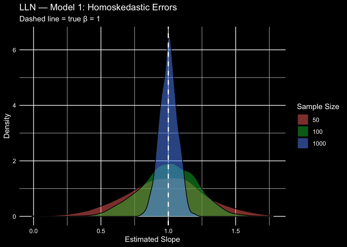
### Model 1: Homoskedastic Errors
$\varepsilon_i \overset{iid}{\sim} \mathcal{N}(0, 1)$. This is the textbook case: errors are well-behaved and identically distributed.
```{r lln-model1}
sim_m1 <- matrix(NA, nrow = length(sample_sizes), ncol = num_simulations)

for (t in seq_along(sample_sizes)) {
  for (s in 1:num_simulations) {
    data    <- gen_data(n = sample_sizes[t], dgp = "model 1")
    reg     <- lm(data$Y ~ data$D + data$X[, 2] + data$X[, 3])
    sim_m1[t, s] <- coef(reg)[2]
  }
}

plot_asympt(sample_sizes, sim_m1) +
  geom_vline(xintercept = 1, color = "white", linetype = "dashed", linewidth = 0.8) +
  labs(title = "LLN — Model 1: Homoskedastic Errors",
       subtitle = "Dashed line = true β = 1")
```
::: {.callout-tip}
## What to look for
As $n$ increases from 50 to 1000, the density concentrates tightly around $\beta = 1$. This is the LLN in action: more data means less variability in the estimate.
:::
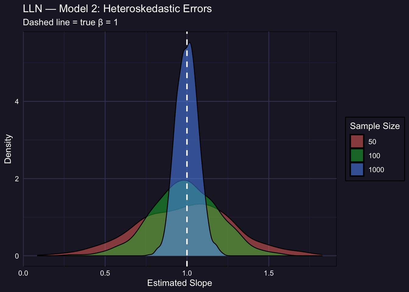
### Model 2: Heteroskedastic Errors
$\varepsilon_i \sim \mathcal{N}(0,\ e^{0.4 X_{2i}})$. The variance of the error now depends on the covariate $X_2$. OLS remains consistent (heteroskedasticity does not cause bias), but the sampling distribution may be wider.
```{r lln-model2}
sim_m2 <- matrix(NA, nrow = length(sample_sizes), ncol = num_simulations)

for (t in seq_along(sample_sizes)) {
  for (s in 1:num_simulations) {
    data    <- gen_data(n = sample_sizes[t], dgp = "model 2")
    reg     <- lm(data$Y ~ data$D + data$X[, 2] + data$X[, 3])
    sim_m2[t, s] <- coef(reg)[2]
  }
}

plot_asympt(sample_sizes, sim_m2) +
  geom_vline(xintercept = 1, color = "white", linetype = "dashed", linewidth = 0.8) +
  labs(title = "LLN — Model 2: Heteroskedastic Errors",
       subtitle = "Dashed line = true β = 1") +
  theme(
      panel.background  = element_rect(fill = "#1e1e2e"),
      plot.background   = element_rect(fill = "#1e1e2e"),
      panel.grid.major  = element_line(color = "#3e3e5e"),
      panel.grid.minor  = element_line(color = "#2e2e4e"),
      text              = element_text(color = "white"),
      axis.text         = element_text(color = "white"),
      legend.background = element_rect(fill = "#1e1e2e"),
      legend.text       = element_text(color = "white"),
      legend.title      = element_text(color = "white"),
      legend.key        = element_rect(fill = NA)
    )
```
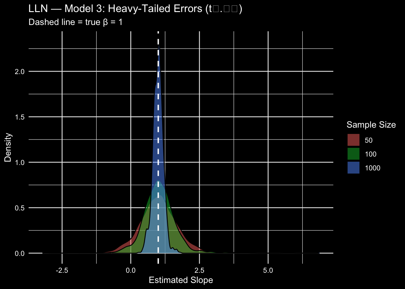
### Model 3: Heavy-Tailed Errors
$\varepsilon_i \sim t_{2.01}$. The $t$-distribution with just over 2 degrees of freedom has very heavy tails — extreme observations are much more likely than under a normal distribution. This is a stress test for the LLN.
```{r lln-model3}
sim_m3 <- matrix(NA, nrow = length(sample_sizes), ncol = num_simulations)

for (t in seq_along(sample_sizes)) {
  for (s in 1:num_simulations) {
    data    <- gen_data(n = sample_sizes[t], dgp = "model 3")
    reg     <- lm(data$Y ~ data$D + data$X[, 2] + data$X[, 3])
    sim_m3[t, s] <- coef(reg)[2]
  }
}

plot_asympt(sample_sizes, sim_m3) +
  geom_vline(xintercept = 1, color = "white", linetype = "dashed", linewidth = 0.8) +
  labs(title = "LLN — Model 3: Heavy-Tailed Errors (t₂.₀₁)",
       subtitle = "Dashed line = true β = 1")
```
::: {.callout-important}
## Heavy tails slow convergence — but do not prevent it
With $t_{2.01}$ errors, the sampling distribution is noticeably wider at $n = 50$ and still somewhat wider at $n = 100$ compared to Models 1 and 2. But by $n = 1000$ the estimates concentrate around $\beta = 1$ just as before. The LLN holds — convergence is just slower when errors are more extreme.
:::
## Summary: Bias and Spread Across DGPs
The table below reports the mean and standard deviation of $\hat{\beta}$ across the 1,000 simulations for each DGP and sample size. A well-behaved estimator should have a mean close to 1 and a standard deviation that shrinks as $n$ grows.
```{r lln-summary-table}
make_summary <- function(sim_mat, label) {
  do.call(rbind, lapply(seq_along(sample_sizes), function(i) {
    data.frame(
      DGP    = label,
      n      = sample_sizes[i],
      Mean   = round(mean(sim_mat[i, ]), 4),
      SD     = round(sd(sim_mat[i, ]), 4)
    )
  }))
}

bind_rows(
  make_summary(sim_m1, "Model 1 (Homoskedastic)"),
  make_summary(sim_m2, "Model 2 (Heteroskedastic)"),
  make_summary(sim_m3, "Model 3 (Heavy tails)")
) %>%
  kbl(caption = "Sampling distribution of β̂ across DGPs and sample sizes",
      col.names = c("DGP", "n", "Mean(β̂)", "SD(β̂)")) %>%
  kable_styling(bootstrap_options = c("striped", "hover"), full_width = FALSE)
```
::: {.callout-note}
## Reading the table
- **Mean(β̂) ≈ 1** across all DGPs and sample sizes: OLS is unbiased (or at least consistent).
- **SD(β̂) decreases with n**: the estimator becomes more precise as we get more data.
- **SD is largest for Model 3**: heavy tails inflate variability, especially at small $n$.
:::