Potential Outcomes: From Theory to Code

Applied Causal Analysis — Coding Exercise

Mauricio Olivares

LMU Munich · Chair of Statistics and Econometrics

2026-04-20

Part I: The Fundamental Problem

What a researcher wishes they could see

Recall from the lecture: for each unit \(i\), we have two potential outcomes

\[Y_i = D_i \cdot Y_i(1) + (1 - D_i) \cdot Y_i(0)\]

but we only ever observe one of \(Y_i(0)\) or \(Y_i(1)\).

Let us make this concrete with a small example.

Generating the Full Schedule of Potential Outcomes

Think of the health care example. We observe \(n = 10\) patients.

n_small <- 10

# Individual treatment effects: β_i ~ N(-0.5, 1)
# Negative on average: hospitalization helps (lower score = better health)
beta <- rnorm(n_small, mean = -0.5, sd = 1)

# Y(0): health score if NOT hospitalised (higher = worse health)
Y0 <- rnorm(n_small, mean = 3, sd = 0.5)

# Y(1): health score if hospitalised
Y1 <- Y0 + beta

Note

\(\beta_i = Y_i(1) - Y_i(0)\) is the individual treatment effect — the quantity we can never directly observe.

The Full Potential Outcomes Table

This is what a god-like researcher would see — both columns at once:

\(i\)	\(Y_i(0)\)	\(Y_i(1)\)	\(\beta_i\)
1	2.05	0.61	-1.44
2	3.46	2.92	-0.54
3	2.78	3.11	0.33
4	3.07	2.14	-0.94
5	2.29	1.47	-0.81
6	2.45	-0.18	-2.63
7	3.64	5.65	2.01
8	3.64	2.02	-1.63
9	2.35	2.02	-0.33
10	2.89	2.96	0.08

Now Assign Treatment — and Watch Data Disappear

# Random assignment: flip a fair coin
D <- rbinom(n_small, 1, 0.5)

# Observed outcome: only ONE potential outcome is revealed
Y_obs <- ifelse(D == 1, Y1, Y0)

\(i\)	\(D_i\)	\(Y_i(0)\)	\(Y_i(1)\)	\(Y_i^{obs}\)
1	0	2.05	NA	2.05
2	1	NA	2.92	2.92
3	0	2.78	NA	2.78
4	1	NA	2.14	2.14
5	0	2.29	NA	2.29
6	0	2.45	NA	2.45
7	0	3.64	NA	3.64
8	0	3.64	NA	3.64
9	1	NA	2.02	2.02
10	1	NA	2.96	2.96

Every ? is a missing counterfactual — this is what makes causal inference a missing data problem.

The True ATE — and Why We Can’t Compute It

# True ATE: we know this only because we simulated the data
ATE_true <- mean(beta)
round(ATE_true, 3)

[1] -0.591

# What a researcher actually computes from observed data
APE <- mean(Y_obs[D == 1]) - mean(Y_obs[D == 0])
round(APE, 3)

[1] -0.3

Warning

With only \(n = 10\) units and random assignment, these two numbers may already differ noticeably. Why? Small samples, not bias. Let us scale up.

Part II: Selection Bias

Scaling Up — and Introducing Selection

We now use \(n = 1{,}000\) units and introduce selection on levels: sicker patients (higher \(Y_i(0)\)) are more likely to seek hospitalisation.

n <- 1000

# Individual treatment effects
beta  <- rnorm(n, mean = -0.5, sd = 1)

# Y(0): baseline health (higher = worse)
Y0 <- rnorm(n, mean = 3, sd = 1)

# Y(1): health if hospitalised
Y1 <- Y0 + beta

A Biased Assignment Mechanism

# Selection on levels: probability of treatment increases with Y(0)
# i.e., sicker people are more likely to go to hospital
p_treat <- plogis(-2 + 1.5 * Y0)   # logistic link
D_sel   <- rbinom(n, 1, p_treat)

# Observed outcomes
Y_sel <- ifelse(D_sel == 1, Y1, Y0)

Fraction treated: 0.85

Mean Y(0) among treated:   3.148

Mean Y(0) among untreated: 1.966

Important

The treated have a higher baseline \(Y_i(0)\) — they are sicker to begin with. This is exactly selection on levels.

The Bias Decomposition — in Code

Recall from the lecture:

\[\underbrace{\mathbb{E}[Y_i|D_i=1] - \mathbb{E}[Y_i|D_i=0]}_{\text{APE (observed)}} = \underbrace{\mathbb{E}[Y_i(1)-Y_i(0)|D_i=1]}_{\text{ATT}} + \underbrace{\mathbb{E}[Y_i(0)|D_i=1] - \mathbb{E}[Y_i(0)|D_i=0]}_{\text{selection bias}}\]

APE_sel <- mean(Y_sel[D_sel == 1]) - mean(Y_sel[D_sel == 0])
ATT_sel <- mean(Y1[D_sel == 1])    - mean(Y0[D_sel == 1])
SB_sel  <- mean(Y0[D_sel == 1])    - mean(Y0[D_sel == 0])
ATE_true <- mean(beta)

The Numbers

Quantity	Value
APE (observed)	0.678
ATT	-0.504
Selection Bias	1.182
ATT + Selection Bias	0.678
True ATE	-0.501

Note

ATT + Selection Bias = APE ✓ — the decomposition holds exactly.

The selection bias is positive: hospitalized patients are sicker to begin with, inflating the observed health gap and masking the true (negative) treatment effect.

Visualising the Selection Problem

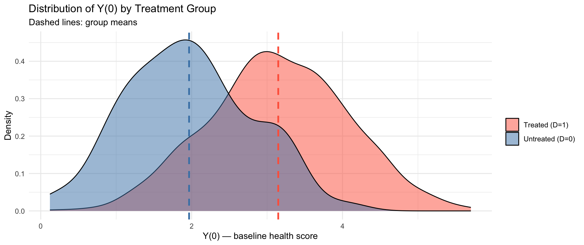
The two distributions of \(Y_i(0)\) are shifted — the treated were sicker before treatment.

Part III: Random Assignment as the Fix

Randomly Assigning Treatment

# Fair coin flip — independent of Y(0) and Y(1)
D_rand <- rbinom(n, 1, 0.5)

# Observed outcomes
Y_rand <- ifelse(D_rand == 1, Y1, Y0)

Mean Y(0) among treated:   2.969

Mean Y(0) among untreated: 2.97

Tip

Under random assignment, the two groups have similar baseline \(Y_i(0)\). Selection bias vanishes.

The Decomposition Under Random Assignment

APE_rand <- mean(Y_rand[D_rand == 1]) - mean(Y_rand[D_rand == 0])
ATT_rand <- mean(Y1[D_rand == 1])     - mean(Y0[D_rand == 1])
SB_rand  <- mean(Y0[D_rand == 1])     - mean(Y0[D_rand == 0])
ATU_rand <- mean(Y1[D_rand == 0])     - mean(Y0[D_rand == 0])

Quantity	Selection on Levels	Random Assignment
APE (observed)	0.678	-0.482
ATT	-0.504	-0.481
ATU	NA	-0.520
True ATE	-0.501	-0.501
Selection Bias	1.182	-0.001
ATT + Selection Bias	0.678	-0.482

Side-by-Side: What Randomisation Fixes

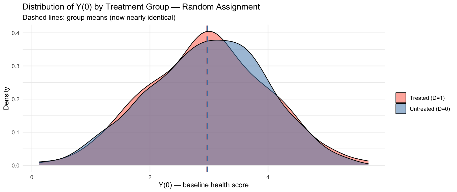
The distributions of \(Y_i(0)\) now overlap almost perfectly. Selection bias \(\approx 0\).

Randomisation Works In Expectation

Does it always work in a single draw? Let us check across many replications:

R       <- 2000   # replications
APE_sim <- numeric(R)

for (r in 1:R) {
  D_r       <- rbinom(n, 1, 0.5)
  Y_r       <- ifelse(D_r == 1, Y1, Y0)
  APE_sim[r] <- mean(Y_r[D_r == 1]) - mean(Y_r[D_r == 0])
}

Mean of APE across 2000 replications: -0.5007

True ATE:                               -0.5012

Sampling Distribution of the APE

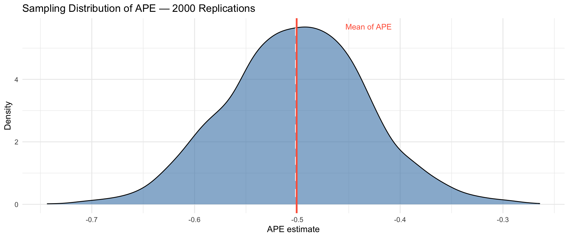
The APE is centred on the true ATE. In any single study there is sampling variability — but the estimator is unbiased.

Part IV: Selection on Gains

A Different Kind of Selection

In-class exercise (Lecture 3, Slide 19)

Show that in general \(\text{ATE} \neq \text{ATT}\) due to selection on gains, but that \(\text{ATE} = \text{ATT}\) under random assignment.

Selection on gains means individuals sort into treatment based on how much they benefit:

\[\mathbb{E}[Y_i(1) - Y_i(0) \mid D_i = 1] \neq \mathbb{E}[Y_i(1) - Y_i(0) \mid D_i = 0]\]

Generating Selection on Gains

# Those who benefit MORE (more negative beta) are more likely to seek treatment
p_gains <- plogis(2 - 3 * beta)    # treatment prob increases as β_i decreases
D_gains <- rbinom(n, 1, p_gains)
Y_gains <- ifelse(D_gains == 1, Y1, Y0)

Mean β_i among treated:   -0.761

Mean β_i among untreated: 0.722

True ATE:                 -0.501

The treated have more negative \(\beta_i\) on average — they are self-selecting because they gain more from treatment.

ATE vs ATT vs ATU Under Selection on Gains

ATE_gains <- mean(beta)
ATT_gains <- mean(beta[D_gains == 1])
ATU_gains <- mean(beta[D_gains == 0])
APE_gains <- mean(Y_gains[D_gains == 1]) - mean(Y_gains[D_gains == 0])
SB_gains  <- mean(Y0[D_gains == 1]) - mean(Y0[D_gains == 0])

Quantity	Value
True ATE	-0.501
ATT	-0.761
ATU	0.722
APE (observed)	-0.710
Selection Bias (levels)	0.051

\(\text{ATE} \neq \text{ATT} \neq \text{ATU}\) — each answers a different causal question.

Random Assignment Restores ATE = ATT

ATT_r <- mean(beta[D_rand == 1])
ATU_r <- mean(beta[D_rand == 0])
ATE_r <- mean(beta)

Quantity	Selection on Gains	Random Assignment
ATE	-0.501	-0.501
ATT	-0.761	-0.481
ATU	0.722	-0.520

Under random assignment, \(D_i \perp (Y_i(0), Y_i(1))\), so who ends up treated is unrelated to their gains — and ATE \(\approx\) ATT \(\approx\) ATU. ✓

Part V: QTE Identification

Beyond Means — Quantile Treatment Effects

Recall from Lecture 3: under random assignment,

\[\underbrace{F_1^{-1}(\tau) - F_0^{-1}(\tau)}_{\text{QTE}_\tau,\ \text{unobserved}} = \underbrace{F^{-1}(\tau \mid D_i=1) - F^{-1}(\tau \mid D_i=0)}_{\text{observed}}\]

Let us verify this numerically.

Computing QTEs

quantiles <- seq(0.1, 0.9, by = 0.05)

# Unobserved QTE: quantiles of potential outcome distributions
qte_true <- quantile(Y1, quantiles) - quantile(Y0, quantiles)

# Observed under random assignment
qte_obs  <- quantile(Y_rand[D_rand == 1], quantiles) -
            quantile(Y_rand[D_rand == 0], quantiles)

# Observed under selection on levels (biased)
qte_sel  <- quantile(Y_sel[D_sel == 1], quantiles) -
            quantile(Y_sel[D_sel == 0], quantiles)

QTE: Random Assignment Identifies the Truth

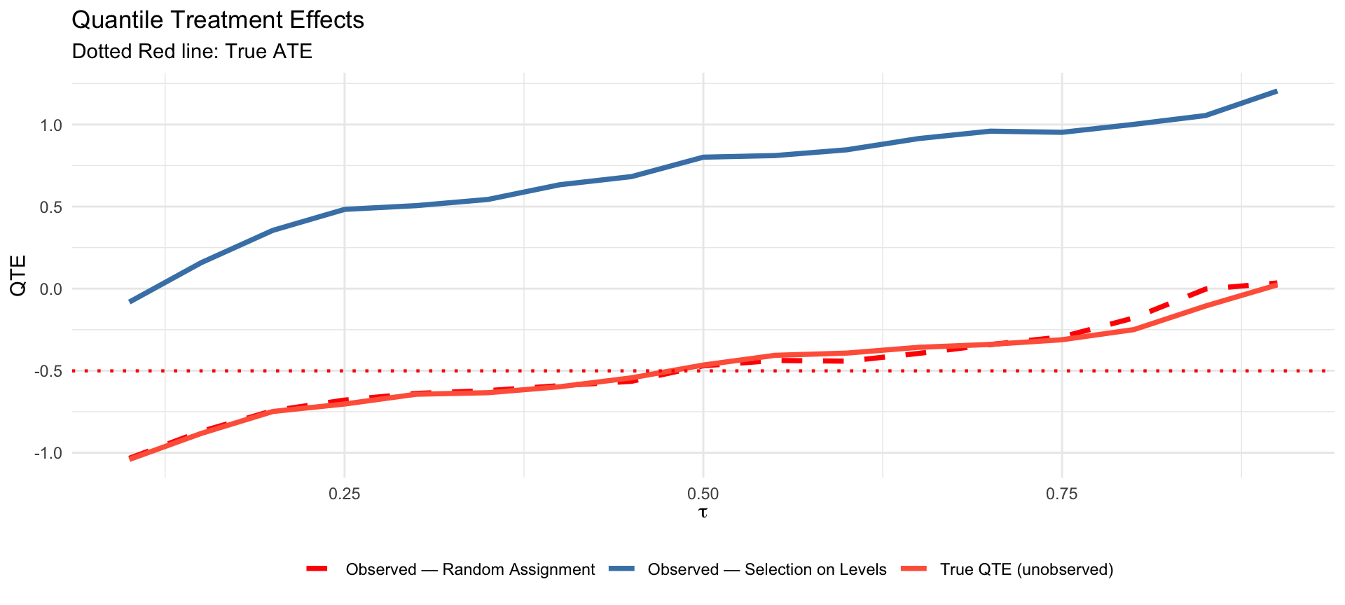
The observed QTE under random assignment (blue) tracks the true QTE closely. Under selection on levels (red) it is systematically distorted.

Summary

What We Did — and Why It Matters

The fundamental problem — with \(n=10\) we saw the missing counterfactual table directly: every ? is what makes causal inference hard
Selection on levels — sicker patients self-select into hospitals; the bias decomposition \(\text{APE} = \text{ATT} + \text{Selection Bias}\) holds exactly in the data
Random assignment — the fix: \(D_i \perp (Y_i(0), Y_i(1))\) kills selection bias, and the APE is unbiased for the ATE across replications
Selection on gains — a subtler problem: ATE \(\neq\) ATT \(\neq\) ATU; random assignment equalises all three
QTE identification — under random assignment, observed quantile differences recover the true QTE; under selection they do not

Looking Ahead

The next step: estimation and inference — how do we attach uncertainty to these estimates?

Standard errors for the difference-in-means
Permutation tests (no asymptotic approximation needed)
Bootstrap inference
Covariate adjustment for efficiency gains

Reading for next class: Lecture 3 slides, sections on covariate balance and the CATE.